Examples

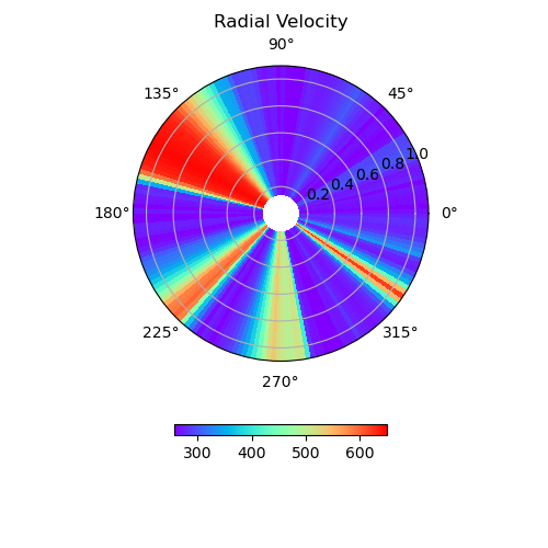
Example #1: Equatorial Slice

import os
import sys
import pysunrunner
import pysunrunner.pload as pp
import pysunrunner.io as io
import pysunrunner.pviz as pviz
import numpy as np
import matplotlib.pyplot as plt
from pathlib import Path
import requests

def download_files(base_url, local_dir):
    if not os.path.exists(local_dir):
        os.makedirs(local_dir)

    # Assuming you have a list of filenames
    filenames = ['dbl.out','Bx1.0000.dbl','prs.0000.dbl','rho.0000.dbl','vx1.0000.dbl','grid.out']
    for filename in filenames:
        url = os.path.join(base_url, filename)
        local_path = os.path.join(local_dir, filename)
        response = requests.get(url)
        with open(local_path, 'wb') as f:
            f.write(response.content)
        print(f"Downloaded {filename}")

base_url = 'http://www.predsci.com/~pete/research/sunrunner/test/output/'
local_dir = './local_files/'

download_files(base_url, local_dir)

time_idx = 0

# Load PLUTO results for this time point
D = pp.pload(time_idx, w_dir=local_dir, datatype='dbl')

# Variable to be plotted
var_name = 'vx1'

# Set polar projection for the plot
subplot_kw = {'projection': "polar"}

# Set color map for the plot (default is 'rainbow')
cmap = 'rainbow'

# Set title for the plot
title = 'Radial Velocity'

# Set log_scale to True for a log10 plot of the data (useful for variables like pressure)
log_scale = False

# Set r_scale to True to apply r^2 scaling (useful for variables like scaled radial magnetic field or density)
r_scale = False

# Create a figure with a single subplot using polar projection
fig, ax = plt.subplots(subplot_kw=subplot_kw, figsize=(5, 5))

# Plot the equatorial cut of the data on the polar projection
axs = pviz.plot_equatorial_cut(D=D, var_name=var_name, ax=ax, cmap=cmap, title=title,
                           r_scale=r_scale, log_scale=log_scale)

plt.show()

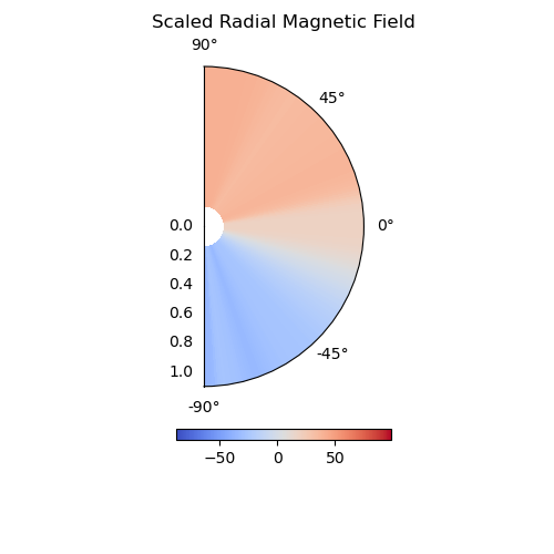
Example #2: Meridonial Slice

import os
import sys
import pysunrunner
import pysunrunner.pload as pp
import pysunrunner.io as io
import pysunrunner.pviz as pviz
import numpy as np
import matplotlib.pyplot as plt
from pathlib import Path
import requests

def download_files(base_url, local_dir):
    if not os.path.exists(local_dir):
        os.makedirs(local_dir)

    # Assuming you have a list of filenames
    filenames = ['dbl.out','Bx1.0000.dbl','prs.0000.dbl','rho.0000.dbl','vx1.0000.dbl','grid.out']
    for filename in filenames:
        url = os.path.join(base_url, filename)
        local_path = os.path.join(local_dir, filename)
        response = requests.get(url)
        with open(local_path, 'wb') as f:
            f.write(response.content)
        print(f"Downloaded {filename}")

base_url = 'http://www.predsci.com/~pete/research/sunrunner/test/output/'
local_dir = './local_files/'

download_files(base_url, local_dir)

time_idx = 0

# Load PLUTO results for this time point
D = pp.pload(time_idx, w_dir=local_dir, datatype='dbl')

# Variable to be plotted
var_name = 'Bx1'

# set phi cut value in degrees.  Here it is set to 295 degrees.
phi_cut = np.deg2rad(295.0)

# Set polar projection for the plot
subplot_kw = {'projection': "polar"}

# Set color map for the plot (default is 'rainbow')
cmap = 'coolwarm'

# Set title for the plot
title = 'Scaled Radial Magnetic Field, phi = '+str(np.rad2deg(phi_cut))

# Set log_scale to True for a log10 plot of the data (useful for variables like pressure)
log_scale = False

# Set r_scale to True to apply r^2 scaling (useful for variables like scaled radial magnetic field or density)
r_scale = True

# convert from code units to nT
b_fac_pluto = 0.0458505

# Create a figure with a single subplot using polar projection
fig, ax = plt.subplots(subplot_kw=subplot_kw, figsize=(5, 5))

# Plot the phi cut of the data on the polar projection
ax = pviz.plot_phi_cut(D=D, var_name = var_name,
    phi_cut = phi_cut, ax = ax,cmap = cmap, title = title,
    r_scale = r_scale, log_scale=log_scale, conversion_units = b_fac_pluto)

plt.show()